Introduction to Statistics and Probability
Chapter 1: Data Collection and Classification
1.1 The Basic of Statistics
Statistics The science of collecting, organizing, analyzing, and interpreting data to make decisions.
An individual refers to a person or object of interest. The collecton of all individuals to be studied is called a population. A sample is a subset of the population being studied.
A parameter is a numerical summary of a population. A statistic is a numerical summary of a sample.
Inferential Statistics Is the process of taking a result from a sample and extending it to the population sampled from while measuring the reliability of the result.
It is often the case that time, money, and resources limit the ability of a researcher to collect data. In these cases, the researcher might consider sampling from the population.
Descriptive Statistcs Involves the organizing and summarizing of data. Some common tools in the process are tables, graphs, and numberical summaries.
It is a very important aspect of research, as it allows us to get an overview of what the data is telling us.
The Process of Statistics
- Identify the research objective.
- Collect the information needed to answer the research objective.
- Describe the data.
- Perform inference.
- Measure the reliability of the inference.
1.2 Data Classification
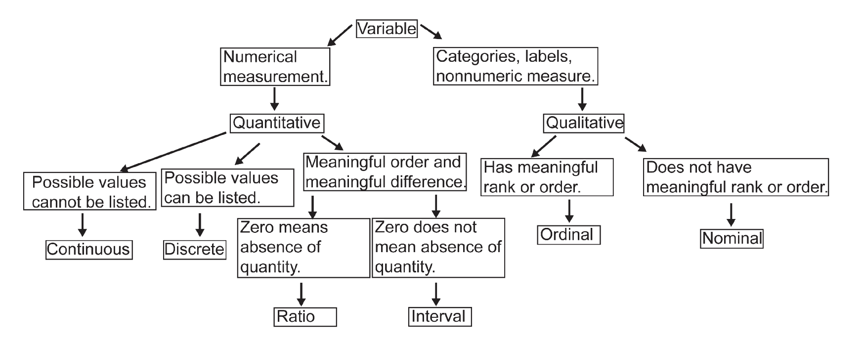
Qualitative (or categorical) variables are variables whose possible values represent categories, labels, etc. that are not numerical measures of counts.
Quantitative variables are variables whose possible values are numerical measurements or counts.
A variable is at the nominal level of measurement if the possible values of the variable represent names, labels, or categories that don't have a meaningful rank or order.
A variable is at the ordinal level of measurement if the possible values of the variable represent names, labels, or categories and have a meaningful rank or order.
When the value of zero means the absence of the quantity, we have an inherent zero.
A variable is at the interval level measurement if the values of variable:
- Have a meaningful order
- Meaningful difference between values
- A value of zero does not mean the absence of the quantity. In this case, we say that the value of zero is not an inherent zero.
A variable is at the ratio level of measurement if the values of the variable:
- Have a meaningful order,
- Meaningful difference between values,
- The value of zero is an inherent zero.
A quantitative variable is discrete if its possible values can be listed. Data only takes certain values. Commonly in the form of whole numbers or integers, this is data that can be counted and has a finite number of values. These values are unable to be broken down into smaller parts.
A quantitative variable is continuous if its possible values cannot be listed. This data can be measured, values are not fixed and have an infinite number of possible values. These measurements can also be broken down into smaller individual parts.
1.3 Simple Random Sampling
Frame: a list of all individuals.
Simple random sampling occurs when every sample of size n from a population of size N is equally likely to be selected.
Sampling with replacement occurs when each individual selected from the population is put back in the population before the next selection (and so could be potentially included in the sample more than once.)
Sampling without replacement occurs when each individual selected from the population is removed from the population before the next selection so that the individual cannot be included in the sample more than once.
1.4 Other Sampling Methods
Convenience sampling is a sampling technique where subjects are selected because of their convenient accessibility to the researcher.
This sampling technique is very popular because it is fast, inexpensive, and easy to do. Unfortunately, studies that use convenience sampling generally cannot be trusted.
Stratified sampling is a sampling technique where the population is separated into disjoint (non-overlapping) groups called strata, and then a simple random sample from each stratum is obtained.
Cluster sampling is a sampling technique where the population is separated into disjoint groups, a simple random sample of groups are selected, and, every individual or a random sample of individuals within the selected groups are observed.
Systematic sampling is a sampling technique where every kth individual in the population is selected after some random start. Usually, the random start is determined by selecting a random number between 1 and k.
1.5 Sample Bias
If the sample is not representative of the population, then the sample has bias...if the sampling technique used tends to favor one part of the population over another, then we have sampling bias.
Nonresponse bias occurs when individuals in the sample do not respond to the survey.
Response bias occurs when the response of an individual in the sample does not reflect the true feelings of the individual.
Chapter 2: Graphical Displays of Data
2.1 Organizing Qualitative Data
A frequency distribution is a table that lists each category of data and shows the number of obervations in each category.
Each category of data is referred to as a class.
The class frequency is the number of observations that fall into that class. The relative class frequency is the proportion of observations that fall into that class.
A relative frequency distribution is a table that lists each category of data and shows the proportion of observations in each category.
Note: The sum of the relative frequencies in a relative frequency distribution must add to 1. However, in practice, this may not be the case due to rounding errors. Again, the order in which the classes are listed, the spaciing, the scaling, and the use of any colors is up to the researcher.
A frequency bar graph is constructed by labeling each category of data on either the horizontal or vertical axis, and its frequency on the other axis. Bars of equal width are drawn for each category, and the height of each bar represents the category's frequency.
A relative frequency bar graph is constructed by labeling each category of data on either the horizontal or vertical axis, and its relaitve frequency on the other axis. Bars of equal width are drawn for each category, and the height of each bar represents the category's relative frequency.
If one orders bars by decreasing height, we have what is called a Pareto chart.
The angle of a class sector in a pie chart, is obtained by mulitplynig 360 degrees by the relative class frequency.
2.2 Organizing Quantitative Data
First, determine if the data is discrete or continuous. If the data is discrete and there are not too many different values, treat each observed data value as a class. If the data is discrete, but there are many different values, then categories of data should be created by using intervals of numbers as the classes.
In the case that the data is continuous, then categories of data should be created using intervals.
A frequency distribution is a table that lists each category (class) of data and shows the number of observations in each category.
Guildine: Generally, there should be between 5 classes (for smaller data sets) and 200 classes (for larger data sets).
Each class has a lower class limit, which is the least number that can belong to the classs, and an upper class limit, which is the greatest number that can belong to the class. The average of the upper class limit and lower class limit is called the class midpoint. The class width is the difference between two consectutive lower class limits, and should be the same for all classes.
Usually, introductory statistics textbooks only address the above terms when dealing with continuous data.
Class boundaries (lower and upper class boundaries) coincide with the midpoints found by averaging each upper class limit with its right neighboring lower class limit. They are the endpoints of touching intervals. Typically, adding and substracting .5, .05, or .005 from the upper/lower class limits repsectively will do the trick.
For example classes, 2-4, 5-7, 8-10. Have lower class boundaries of 1.5, 4.5, 7.5 and upper class boundaries of, 4.5, 7.5, 10.5.
Limits = inclusive Boundaries = exclusive
Class frequency is the number of observations that fall into that class. Relative class frequency is the proportion of observations that fall into that classs.
A relative frequency distribution is a table that lists each category of data and shows the proportion of observations in each category.
A histogram is similar to a bar graph, except that the rectangles in histograms touch, while the bars in bar graphs do not touch. When the vertical scale measures the frequencies of the classes, we have a frequency histogram. When the vertical scale measures the relative frequencies of the classes, we have a relative frequency historgram.
2.3 Additional Displays of Quantitative Data
The cumulative frequency of a class is the sum of the frequency of that class and the frequencies of all previous classes.
The cumulative relative frequency of a class is the sum of the relative frequency of that class and the relative frequencies of all previous classes.
A dot plot is a graphical display of data drawn by placing each observation horizontally on a number line and placing a dot above the observation for each time it is observed.
In a stem and leaf plot, each number is separated into a stem (digits left of the rightmost digit) and a leaf (the rightmost digit). Stems are written in a single vertical column, and a vertical bar to the right of that column is drawn, and each leaf is written to the right of the vertical bar in the row corresponding to its stem.
// e.g.
10.2 -> 10 (stem) | 2 (leaf)
112 -> 11 (stem) | 2 (leaf)
2.4 Shapes of Distributions
A frequency distribution is symmetric when a vertical line can be drawn through the middle of the graph of the distribution, and the resulting halves are mirror images of each other.
A frequency distribution is uniform when all classes in the distribution have equal frequencies. A frequency distribution that is shaped like a bell is called bell-shaped.
(single peak assumed) Skewed left (negatively skewed): left tail is longer than right tail. Skewed right (positively skewed): right tail is longer than left tail.
Qualitative data is not described as uniform, bell-shaped, or skewed, since the order in which the classes are displayed is arbitrary. We only use these terms to describe quantitative data.
Data will probably not perfectly match one of the four descriptions, so we use "approximately" symmetric/uniform/etc. to describe.
The shape of the distribution is often times subjective (especially since changing the class width and number of classes used in a frequency distribution can drastically change the shape of the histogram). The terms are introduced informally, not precisely, for the benefit of exposure to the terms.
Bidmodal: having two peaks.
For these notes, if a distribution is not unimodal, we will not attempt to classify the shape.
3.1 Measures of Central Tendency
A sample dataset is written with a lowercase n.
n = 5
A population dataset is written with an upperecase N.
N = 5
Most introductory stats textbooks drop the sigma sub/superscripts and just write Σ x = ..., which is interpreted as "the sum of all oberservations in the data set". Dropping the sub/superscripts makes it unclear whether the data set represents a sample or a population.
Example 1:
Consider the data set: {10, 11, 11, 13, 14}
Evaluate: Σ x
Solution:
Σ x means "add all of the observations in the data set".
Σ x = 59
Example 2:
Consider the data set: {10, 11, 11, 12, 13}
Evaluate: Σ x/2
Solution:
Σ x/2 means "divide each observation by 2, then add them all".
Σ x/2 = 28.5
It turns out, Σ x/2 is equivalent to (Σ x)/2.
Arithmetic mean is the sum of data values divided by the number of data values — in everyday parlance we refer to this as the mean.
x̄, pronounced X bar, represents the sample mean.
μ represents the population mean.
x̄ = Σ x/n is considered a statistic, b/c it involves the sample.
μ = Σ x/N is considered a parameter, b/c it involves the population.
The median is found via taking the middle value when arranged from lowest to highest. If there are an even number of observations, then the mean of the two middle values is used.
There is no widely accepted standard symbol for the median.
The mode of a data set (quantitative or qualitative) is the data value of the highest frequency. If no data value is repeated, the data has no mode.
There are other interpretations of the mode in terms of local maximums of a frequencyy distribution which can allow for more than one mode, bimodal, trimodal, or multimodal.
The weighted mean of a quantitative data set is similar to the mean of the data set, except that the data values are assigned weights.
(Σ wi * xi) / Σ wi
Meaning, multiply each data value by its weight, add them up, then divide that sum by the sum of the weights.
Example given data set, { 10, 20, 30, 40 } and weights, { 20, 20, 40, 20 }.
// sigma (weight * data value) / sigma weights

(20*10 + 20*20 + 40*20 + 20*40) / 20 + 20 + 40 + 20

= 2600 / 100
= 26
Often, a course will use a weighted average to calculate final class grades. E.g 15% from your mean homework, 15% from quizes, and 70% from the final exam.
// weights: 15, 15, 70
// grades: 85, 90, 82

(15*85 + 15*90 + 70*82) / 100

= 83.65
A measure of central tendency is a single value that attempts to describe a set of data by identifying the central position within a data set.
We say that a measure of central tendency is resistant if extreme values relative to the data do not affect its value substantially.
The median and mode are resistant to extreme values (outliers), but the mean is not.
Aside: Other means exist including, the geometric mean, harmonic mean, generalized mean (power mean), f-mean, truncated mean, etc.
10 + 22 + 33 + 44 / 10
3.2 Measure of Dispersion
Statistical dispersion refers to how stretched or squeezed the data are. Measures include:
- Range
- Standard Deviation
- Variance
- Interquartile range
- Median absolute deviation
- Average absolute deviation
Range
range = greatest value - least data value
- Can never be negative
- Is in same units as the data
- Sample range, population range, or simply range
- Is generally not sufficient to describe the spread of data.
- Is not resistant to extreme values.
Deviation about the mean is equal to the ith data value minus the mean of the data set.
// sample
di = xi - x̄

// population
di = xi - μ
The sum of deviations about the mean and the mean of deviations about the mean are both zero.
Using absolute values of deviations about the mean is a way to circumvent zero sums, and work with/find central tendencies with deviations. These can be described with:
- Mean absolute deviation
- Median absolute deviation
Absolute deviations prevent positive deviations from canceling negative deviations. Another way to prevent this is to square deviations about the mean.
Sample variance
(Σ (x - x̄)^2) / n - 1
Population variance
(Σ (x - μ)^2) / N
The sample standard deviation is defined as the square root of the sample variance, and we use the symbol s to denote it. The population standard deviation is defined as the square root of the population variance, and we use the symbol σ to denote it.
We use n - 1 in the denominator for sample variation and sample standard deviation. This results in an overestimate of values, some would say an approximatation of said values. This is not true for population variance and standard deviation.
Standard deviation is the sqaure root of the variance. Standard deviation can be larger that variance when working with variances less than one, e.g.
- variance = 1/4, std deviation = 1/2 AKA the sqaure root of 1/4 = 1/2
The Empirical Rule
If a distribution is roughly bell shaped, then:
- ~68% of the data will lie within 1 std deviation of the mean (
μ - 1σandμ + 1σ) - ~95% will lie within 2σ
- ~99.7% will lie within 3σ
This is also true for sample data, x̄.
Chebychev's Rule
For any data set, regardless of the shape of the distrubution;
- At least 75% of the data will lie within 2 std deviations of the mean
- At least 88.9% of the data will lie within 3 std deviations of the mean
- At least
(1 - 1/k^2)100%of the data will lie within K standard deviations of the mean for k > 1. That is, at least(1 - 1/k^2)100%of the data will lie betweenμ - kσandμ + kσ
This is also true for sample data, x̄.
3.3 Measures of Central Tendency and Dispersion From Grouped Data
Approximating the Mean from a Frequency Distribution
- Multiply each class midpoint by its class frequency.
- Sum all the products calculated in step 1.
- Sum all the class frequencies to obtain the total number of data values in the data set.
- Divide the sum in step 2 by the sum in step 3.
(Σ mi * fi) / Σ fi
Approximating the Variance from a Frequency Distribution
- Calculate the mean.
- Calculate the squared deviations.
- Multiply each squared deviation by its corresponding class frequency.
- Sum all products from step 3.
- Sum all the class frequencies.
- If the data set represents a population, divide by sigma class frequencies. If the data set represents a sample, divide by sigma cf - 1.
sample variance = (Σ (mi - x̄)^2 * fi) / (Σ fi) - 1
population variance = (Σ (mi - μ)^2 * fi) / (Σ fi)
To approximate the standard deviation from a frequency distribution, simply take the square root of the variance (see above).
3.4 - Measures of Relative Standing
Measures of relative standing are numbers which indicate where a particular value lies in relation to the rest of the values in a data set. There are many different measures of relative standing, but we will just cover the two most common measures in statistics: z-scores and quartiles.
The z-score of a data value represents the number of standard deviations the data value is away from the mean of the data set.
// sample z-score
(x - x̄) / S

// population z-score
(x - μ) / σ
- If z-score is negative, x is less than the data set
- If z-score is positive, x is more than the data set
- If z-score is zero, x is the mean of the data set
The kth percentile of a data set is a value such that k percent of the data values are less than or equal to the value.
Quartiles are a special case of percentiles.
- Q1 25th, Q2 50th AKA the median, Q3 75th percentiles
To find quartiles:
- Arrange data in ascending order
- Find the median (second quartile)
- Divide the data set into 2 halves
- The 1st and 3rd quartiles will be the median of the lower and upper halves respectively
- Do not include (n + 1) / 2 AKA step 2in either half.
^ This definition of quartiles is widely held but not only held.
3.5 - The Five Number Summary and Boxplots
The interquartile range, denoted IQR, is the range of the middle 50% of the data values in a data set.
IQR = Q3 - Q1
The lower fence and upper fence are defined as follows: Lower fence = Q1 - 1.5(IQR) Upper fence = Q3 + 1.5(IQR)
If a data value is less than the lower fence or greater than the upper fence, it is considered an outlier.
The Five number Summary
The range, std, and variance of a data set are not resistant to extreme values. The interquartile range, however, is resistant.
Q1-3 do not provide any information about the extreme values of the data set. One way to obtain this information is to determine the minimum and maximum values in a data set.
The five number summary consists of:
- minumum data value
- Q1
- Q2 (median)
- Q3
- maximum data value
Drawing a Boxplot
- Determine the lower and upper fences
- Draw vertical lines at Q1, Q2, Q3 and enclose the lines in the box
- Draw a horizontal line through the middle of the box, from lowest to greatest data values interior to the fences (the whiskers)
- The 1st value to the right of the lower fence
- The 1st value to the left of the upper fence
- Draw small verticle lines to cap the horizontal line in step 3
- Any outlierers are marked with a small circle. (outside the lower and upper fences)
Some refer to the boxplot as a box-and-whisker plot.
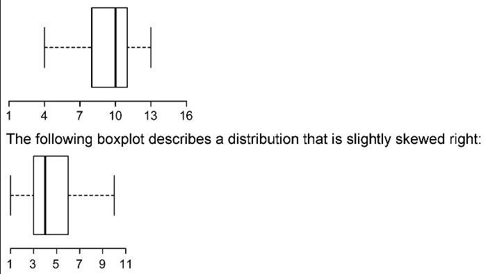
A boxplot gives us a good description of the spread and variability of a data set as well as some idea about the shape of the distribution; particularly if a data set is skewed.
4.1 - The Basics of Probability
In probability theory, an experiment is any procedure with uncertain results that can be repeated and has a well-defined set of possible outcomes known as the sample space.
An event is any collection of outcomes (one or more) from a probability experiment.
Probability is a measure of the likelihood of the occurrence of an event.
There are three type of probability that we will discuss:
- Classical (theoretical) probability
- Emperical probability
- Subjective probability
If an experiment has n equally likely outcomes, we define the probability of each outcome to b 1/n.
The probability of an event E is defined to be the number of outcomes in the event that belong to the sample space divided by n.
We use the notation P(E), which is read, "P of E" or "the probability of E" to denote the probability of the event E.
// In other words...
// (Think of E as a collection of outcomes, i.e. a subset of the sample space.)
P(E) = Number of possible outcomes in the event E / Total number of outcomes in the sample space
- If
P(E) = 0, thenEis an event that is impossible to occur. In this case, we call teh eventEanimpossible event. - If
P(E) = 1, thenEmust occur with certainty — acertain event. - If
P(E) < 0.05, thenEis considered unlikely to occur — anunusual event.
The emperical probability of an event is the ratio of the number of trials in which the event occured, divided by the total number of trials performed.
Subjective probability is a probability derived from an individual's personal judgment about the likelihood that an event occurs. Subjective probabilities contain no formal calculations and only reflect the subject's opinions and past experience.
The Law of Large Numbers: As the number of repetitionss of a probability experiment increases, the proportion with which a certain outcome is observed gets closer to the classical (theoretical) probability of the outcome.
4.2 The Addition and Complement Rule
Two events are mutually exclusive (disjoint) if they have no outcomes in common. In other words, if one event occurs, the other event cannot occur.
A ∩ B - "A and B", the intersection of A and B. All outcomes in both A and B.
A ∪ B - "A or B", the union of A and B. All outcomes in A, B or both, none counted twice.
The addition rule = A ∪ B = P(A) + P(B) - P(A ∩ B)
^ Can be seen in a venn diagram.
The complement of an event A is the event that A does not occur, A^c.
A ∪ A^c equals the entire sample space.
The complement rule = P(A^c) = 1 - P(A)
4.3 Conditional Probability and The Multiplication Rule
A conditional probability is the probability of an event occurring, given that another event has already occured.
The notation P(A|B) is read, "the probability of A, given event B" and it is the probability that event A occurs, given that B has already occured.
- Conditional probability can be calculated by reducing the sample space, assuming that event B has occured.
- Another way to calculate conditional probability is to use the following formula on the unreduced sample space.
P(A|B) = P(A ∩ B)) / P(B)
Independence test (given event has no bearing on next event):
P(A|B) = P(A)- given
B,P(A)equalsP(A)alone
- given
P(B|A) = P(B)- given
A,P(B), equalsP(B)alone
- given
Two events are independent, provided that the occurence of one event does not affect the probability that the other event occurs. In other words,
P(A|B) = P(A) or P(B|A) = P(B). If one of these equations is not satisified, then the events are dependent. (Note only 1 of the 2 equations needs to be satified to determine independence or dependence. This is because the truth status of one equation implies the truth status of the other equation.)
The multiplication rule states that when events are independent, P(A∩B) = P(A)P(B).
Ex. A is observing heads and B is observing heads, P(A∩B) = P(A)P(B) = .25.
When events are dependent:
- MR1:
P(A∩B) = P(A|B)P(B) - MR2:
P(A∩B) = P(B|A)P(A)
Note, be careful when declaring that two events are independent. Use the mathematical definition of independence, not your intuition. It is possible for two events to be independent in one sample space, but dependent in another sample space.
4.4 Introduction to Combinatorics
The multiplication principle: If there are m ways of performing a task and n ways of performing another task, then there are m * n ways of performing both tasks in sequence.
How many 2 digit codes are possible if the digits come from the set { 0, 1, 2, 3, 4, 5, 6, 7, 8, 9, 10 }?
10 for the 1st digit and 10 for the 2nd digit. 10 * 10 = 100 according to the multiplication principle.
With rules excluding 0 for the 1st digit and disallowing same-digit for the 2nd, we get 9 * 9 = 81.
A permutation is an ordered arrangement of objects. The number of distinct permutations of n distinct objects is n!.
n! is read "n factorial" and is defined as: n! 1 * 2 *** n for all natural numbers n.
We define 0! to be 1.
How many differenct permutations (arrangments) of string abc are there?
3 factorial. 3! = 1 * 2 * 3 = 6
Another formula to find permutations:
n Permuations r order matters
nPr = n! / (n - r)!
n Combinations r order does not matter, ab = ba
nCr= n! / (n - r)!r!
The number of arrangments of r objects taken from n objects.
Permutations with Non-distinct Objects AKA Distinguishable Arrangements
n1 ... nk are of differeing kinds.
n! / n1! * n2! * n3! .. nk!
How many permutations of the word "boo" are there?
n = 3 (3 letters)
kinds:
n1 = b = 1
n2 = o = 2
3! / 1!2!
7 balls, 2 blue, 3 red, 2 yellow
7! / 2!3!2!
`
Citation
westcottcourses.com